Cinematic Color

Content

Cinematic Color

From Your Monitor to the Big Screen
A VES Technology Committee White Paper, Oct 17, 2012

Description

This paper presents an introduction to the color pipelines behind modern feature-film visual-effects and animation.

Color impacts many areas of the computer graphics pipeline. From texture painting to lighting, Rendering to compositing, and from image display to the theater, handling color is a tricky problem. We present an introduction to color science, color encoding, and a discussion of scene-referred and display- referred colorimetry. We then extend these concepts to their use in modern motion-picture color management. Finally, we will present a brief introduction to recent efforts on digital color standardization in the motion-picture industry (ACES and CDL), and how readers can experiment with all of these concepts for free using open-source software (OpenColorIO).

Authorship

This paper was authored by Jeremy Selan and reviewed by the members of the VES Technology Committee including Rob Bredow, Dan Candela, Nick Cannon, Paul Debevec, Ray Feeney, Andy Hendrickson, Gautham Krishnamurti, Sam Richards, Jordan Soles, and Sebastian Sylwan.

Introduction

Practitioners of visual effects and animation encounter color management challenges which are not covered in either traditional color-management textbooks or online resources. This leaves digital artists and computer graphics developers to fend for themselves; best practices are unfortunately often passed along by word of mouth, user forums, or scripts copied between facilities.

This document attempts to draw attention to the color pipeline challenges in modern visual effects and animation production, and presents techniques currently in use at major production facilities. We also touch upon open-source color management solutions available for use at home (OpenColorIO) and an industry attempt to standardize a color framework based upon floating-point interchange (ACES).

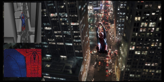
*This fully computer-generated image touches upon many modern techniques in color management, including a scene-linear approach to Rendering, shading, and illumination, in addition to on-set lighting reconstruction and texture management1. Visual effects by Sony Pictures Imageworks. Images from The Amazing Spider-Man Courtesy of Columbia Pictures. ' 2012 Columbia Pictures Industries, Inc. All rights reserved.

This image, though dark, has good detail in the shadows. If these shadow areas appear flat black, please confirm your display calibration and gamma.

What color management challenges are faced in visual effects and animation production?

Various Requirements: It is difficult to lump all of visual effects and animation into a single bucket, as each discipline has potentially differing color pipeline goals and constraints. For example, in visual effects production one of the golden rules is that image regions absent visual effects should not be modified in any way. This places a constraint on color pipelines - that color conversions applied to the photography must be perfectly invertible. Animation has its own unique set of requirements, such as high-fidelity handling of saturated portions of the Color gamut. Thus, color pipelines for motion pictures must keep track of the big picture priorities, and are often tailored to specific productions.

Various Color Philosophies: There are many schools of thought on how to best manage color in digital motion-picture production. (We assert there is far more variation in motion-picture color management than in desktop publishing). Some facilities render in high-dynamic range (HDR) color spaces. Other facilities prefer to render in low-dynamic range (LDR). Some facilities rely on the output display characteristics (i.e., gamma) as the primary tool in crafting the final image appearance. Others do not. It is challenging to provide standardized workflows and toolsets when current practice has such variation.

Furthermore, the costs vs. benefits of adapting new color management techniques is often stacked against change. When something goes wrong in a motion-picture color pipeline, it can have potentially large financial consequences if work needs to be re-done. Furthermore, while color processing decisions are made early during the lifetime of a production, the consequences (both positive and negative) may not be evident until many months down the line. This decoupling of cause and effect makes experimentation and innovation challenging, and all too often leads people to assert We ve always done it this way, it s not worth trying something new.

The flip-slide is that the computer graphics techniques used in motion-picture production are rapidly changing, outgrowing many classic color management techniques. For example, the recent trend toward physically-based rendering, physically-based shading, and plausible lighting models are only utilized to their fullest extent when working with dynamic ranges typical of the real world (HDR). We thus assert that going forward, it will become increasingly beneficial for computer graphics applications and visual- effects and animation facilities to consider modern approaches to color management. Of course, just because a color management technique is new and shiny does not imply superiority. Care must be taken when adopting new approaches to preserve the benefits of the historic color pipelines to the greatest extent possible.

Multiple Inputs & Outputs: In live-action visual effects imagery is often acquired using a multitude of input capture devices (digital motion picture cameras, still cameras, etc) and it is often desired to seamlessly merge sources. On the output side, the final image deliverables are often tailored to distinct viewing environments: digital theatrical presentation, film theatrical presentation, as well as home theater. Each of these outputs has different color considerations. Furthermore, artists often work on desktop displays with office viewing conditions, yet require a high-fidelity preview of the final appearance.

Complex Software Ecosystem: Another challenge is that the majority of visual effects and animation productions use many software tools: image viewers, texture/matte painting applications, composting applications, lighting tools, media generation, etc). Although it is imperative that artists work in a color managed pipeline across multiple applications, color support is quite varied between software vendors. Ideally, all software tools that interchange images, perform color conversions, or display images should be color managed in a consistent manner. The issue of interchange takes on an even more complex angle when you consider that multiple facilities often share image assets on a single film. Color management practices that encourage high-fidelity interchange are sorely needed.

Robust Imagery: Visual effects and animation are not the end of the line in terms of image processing. Digital intermediate (DI) is a powerful tool for crafting the final appearance of a motion-picture (even for animated features) and may substantially impact the appearance of the final film. It is therefore a necessity to create computer graphics which are robust to such workflows, and maintain fidelity even under drastic color corrections. If digital intermediate is not considered during production, it is very likely that late stage color corrections will reveal latent problems in the computer-generated imagery. The eventual application of compression is also a consideration.

Future-Proof: Future improvements to display technology (such as wider dynamic range) are on the near horizon. For large productions, it is very prudent to take all steps possible to future-proof the computer generated imagery, such that you are only a remaster away from taking advantage of the new technology.

Color Science

While a detailed overview of colorimetry is beyond the scope of this document, there are many textbooks which introduce color science in wonderful detail:

Measuring Color [Hunt, 1998] is a compact overview of color measurement and color perception.
Color Imaging: Fundamentals and Application [Reinhard, et al. 2008] presents a ground-up view of color fundamentals, and also covers modern concepts including camera and display technology.
Color Science [Wyszecki and Stiles, 1982] is the canonical bible for color scientists.

A Brief Introduction to Color Science

Color science blends physical measurement along with characterizations of the human visual system. The fundamentals of colorimetry (the measurement and characterization of color) provide an important conceptual framework on which color management is built. Without color science, it would not be possible to characterize displays, characterize cameras, or have an understanding of the imaging fundamentals that permeate the rest of computer graphics. While it is possible to immediately jump into color pipeline implementations, having a rudimentary understanding of concepts such as spectral measurement, XYZ, and color appearance provide a richer understanding of why particular approaches to color management are successful. Furthermore, being familiar with the vocabulary of color science is critical for discussing color concepts with precision.

A study of color science begins with the spectrum. One measures light energy as a function of wavelength. The human visual system is most sensitive to wavelengths from 380-780 nm. Light towards the middle of this range (yellow-green) is perceived as being most luminous. At the extremes, light emitted above 780 nm (infrared) or below 380 nm (ultraviolet) appears indistinguishable from black, no matter how intense.

Wavelength (nm)
The electromagnetic spectrum from approximately 380-780 nm is visible to human observers.²

² Other animals can perceive light outside of this range. Bees, for example, see into the ultraviolet. And imaging devices such as digital cameras typically include internal filtration to prevent sensitivity to infrared.

The human visual system, under normal conditions, is trichromatic³. Thus, color can be fully specified as a function of three variables. Through a series of perceptual experiments, the color community has derived three curves, the CIE 1931 color matching functions,** which allow for the conversion of spectral energy into a measure of color. Two different spectra which integrate to matching XYZ values will appear identical to observers, under identical viewing conditions. Such spectra are known as metamers. The specific shape of these curves is constrained⁴; based upon the results of color matching experiments.

³ For the purposes of this document we assume color normal individuals (non color-blind), and photopic light levels (cone vision).
⁴ These the curves serve as the basis functions for characterizing a human s color vision response to light; thus all linear combinations of these color matching functions are valid measures of color. This particular basis was chosen by locking down Y to the measured photopic luminance response, and then picking X and Z integration curves to bound the visible locus within the +X, +Z octant.

The CIE 1931 Color Matching Functions convert spectral energy distributions into a measure of color, XYZ. XYZ predicts if two spectral distributions appear identical to an average ⁵ human observer.

⁵ The Color Matching Functions are derived from averaging multiple human observers; individual responses show variation. While broad-spectrum light sources have historically not accentuated user variation, the shift to narrow- spectrum/wide-gamut display technologies reveals may increasingly reveal the latent variations in color perception.

When you integrate a spectral power distribution with the CIE 1931 curves, the output is referred to as CIE XYZ tristimulus values, with the individual components being labelled X, Y, and Z (the capitalization is important). The Y component has special meaning in colorimetry, and is known as the photopic luminance function. Luminance is an overall scalar measure of light energy, proportionally weighted to the response of human color vision. The units for luminance are candelas per meter squared (cd/m²), and are sometimes called nits in the video community. The motion-picture community has historically used an alternative unit of luminance, foot-lamberts, where 1 fL equals 3.426 cd/m². A convenient trick to remember this conversion is that 14.0 fL almost exactly to 48.0 cd/m², which coincidentally also happens to be the recommended target luminance for projected theatrical white.

Note that XYZ does NOT model color appearance. XYZ is not appropriate for predicting a spectral energy distribution’s apparent hue, to determine how colorful a sample is, or to determine how to make two color spectra appear equivalent under different viewing conditions⁶. XYZ, in the absence of additional processing, is only sufficient for predicting if two spectral color distributions can be distinguished.

⁶ Color appearance models, far more complex than simple integration curves, model eccentricities of the human visual system and be used to creating matching color perceptions under differing conditions. One of the most popular color appearance model is CIECAM02. See [Fairchild, 98] for details.

CIE XYZ is calculated by multiplying the energy in the input spectrum (top) by the appropriate color matching function (middle), and then summing the area under the curve (bottom). As the color matching functions are based upon the sensitivities human color vision, the spectral energy during integration is zero-valued outside the visible spectrum.*

Spectroradiometers measure spectral power distributions, from which CIE XYZ is computed. By measuring the spectral energy, such devices accurately measure colorimetry even on colors with widely different spectral characteristic. Spectroradiometers can also be pointed directly at real scenes, to act as high fidelity light-meters. Unlike normal cameras, spectroradiometers typically only measure the color at a single pixel , with a comparatively large visual angle (multiple degrees for the color sample is common). Internally, spectroradiometers record the energy per wavelength of light (often in 2, 5, or 10 nm increments), and integrate the spectral measurements with the color matching functions to display the XYZ or Yxy tristimulus values. The exposure times of spectroradiometers are such that color can be accurately measured over a very wide range of luminance levels, in addition to light output with high frequency temporal flicker (such as digital projector). While spectroradiometers are thus incredibly useful in high-fidelity device characterization and calibration, they maintain laboratory-grade precision and repeatability, and are priced accordingly.

Cinematic_Color_010.png|200 Cinematic_Color_011.png|200

Spectroradiometers (left) accurately measure the visible spectrum and can also output an integrated CIE XYZ. Alternative approached to measuring color such as the colorimeter puck (right) are far more cost-effective but do not record the full color spectra. Such devices therefore are only color accurate when tuned to a specific class of display technology. Images courtesy Photo Research, Inc., and EIZO.

It is often convenient to separate color representations into luminance and chroma components, such that colors can be compared and measured independent of intensity. The most common technique for doing so is to to normalize Cap X, Y, Z by the sum (X+Y+Z) and then to represent color as (x, y, Y). Note the capitalization.

\begin{array}{r} x = \frac{X}{X + Y + Z} y = \frac{Y}{X + Y + Z} \end{array}

The Chromaticity coordinates (x,y) define color independent of luminance. It is very common to plot these values, particularly when referring to display device gamuts.

"Little x, little y" (x,y) is referred to as the Chromaticity coordinates, and is used to plot color independent of luminance. When one converts all possible spectra into x,y,Y space and plots x,y they fall into a horse-shoe shaped region on the Chromaticity chart. The edge of the horseshoe is called the visible locus, and corresponds to the most saturated color spectra that can be created. In this chart, luminance (Y) is plotted coming out of the page, orthogonal to x,y. brucelindbloom.com is a wonderful online resource for additional color conversion equations.

Cinematic_Color_68.png|500

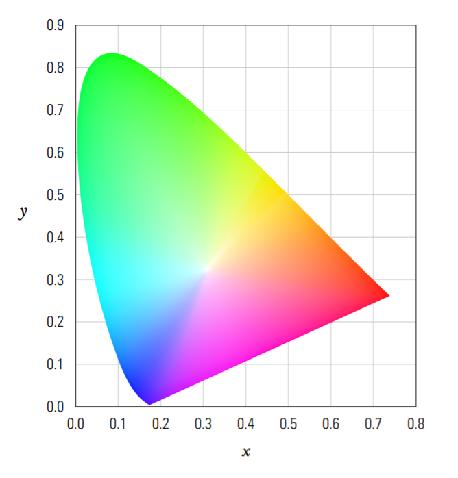
All possible light spectra, when plotted as xy Chromaticity coordinates, fill a horseshoe-shaped region. The region inside the horseshoe represents all possible integrated color spectra; the region outside does not correspond to physically-possible colors. Such non-physically plausible Chromaticity coordinates are often useful for mathematical encoding purposes, but are not realizable in ANY display system.

Additive display systems such as television create colors by blending three colors of light. Red, green, and blue are most often used, as these allow for much of the visible gamut to be reproduced. The gamut of colors that can be reproduced is the triangle enclosed by the primaries. Note that because the outer boundary of horseshoe is curved, there is no possible choice of three colors which encloses the full visible gamut. (Remember, you cannot build real displays with primaries outside of the horseshoe). This is why some recent television manufactures have begun to experiment with adding a fourth color primary.

Although it is not immediately apparent, the Chromaticity chart has very poor perceptual uniformity. The distances between colors in Chromaticity space do not directly relate to their apparent perceptual differences. Two colors nearby in xy may be perceived as appearing very dissimilar, while colors colors far apart may be perceived as being indistinguishable. See MacAdam ellipses in traditional color textbooks for precise graphics representations of this non-uniformity. Roughly speaking, saturated green colors in xy space are over-accentuated relative to their perceptual similarity. The perceptual nonuniform of XYZ (and xy) is not surprising given that XYZ does not model color appearance. One color space that does attempt to create a perceptually uniform color space is CIE L*u*v*, which is calculated using XYZ as an input. While a full discussion of L*u*v* (and more modern alternatives) is outside the scope of this document, when visualizing color gamuts keep in mind that a uv plot is often more informative than the equivalent xy Chromaticity diagram.

Finally, as color is inherently a three dimensional quantity, any discussion which makes use of two dimensional charts tends to be misleading. For a 3-D graphical exploration of CIE XYZ, see Visualizing the XYZ Color Space [Selan 2005].

Color Encoding, Color Space, and Image States

Thus far we have discussed the measurement of color, but have not tied these measurements back to seemingly familiar computer graphics concepts such as RGB. So what is RGB?

RGB is a color encoding where red, green, and blue primaries are additively mixed to reproduce a range (gamut) of colors. The specific color appearance of pure red, green, and blue is tied to the chosen display device; often identified using Chromaticity coordinates. The code values sent to a display device often correspond non-linearly to the emitted Light output, as measured in XYZ. This non-linearity was originally a consequence of display technology, but today serves a continued purpose in increasing the coding efficiency of the transmitted images.

All RGB colors have units. Sometimes an RGB pixel s units are explicit, such as measuring the emitted Light from a display using a spectroradiometer and being able to reference pixel values in XYZ cd/m2. However, sometimes the units are only indirectly related to the real world, such as providing a mathematical conversion to measurable quantities. For example, having code values represent either the logarithm or exponent of RGB is common. This definition of how measurable color quantities relate to image RGB code values is referred to as the color encoding, or more commonly in the motion-picture computer graphics community, color space⁷. In the case of display technology, common color encodings (relations of code value to measurable XYZ performance) include sRGB and DCI-P3.

⁷ The color science community looks down upon the use of color space to denote RGB encodings; color space is strictly preferred to refer to the broader class of color encoding, examples of which are RGB, CMY, HSV, L*a*b*, etc.). However, the mis-use of the color space is so ubiquitous in film production that that we will reluctantly adhere to industry convention.

Considering image display only provides part of the color encoding story. In addition to relating RGB values to display measurements, one can also relate RGB values to the performance characteristics of an input device (i.e., a camera). Input colorimetry can be measured in real world units as well. It is not difficult to measure an input spectra with the spectrophotometer in XYZ, and then compare this to the RGB values output from the camera. This process, called camera characterization, will be discussed further in section 2.3.

It is a meaning abstraction to categorize color spaces by the direction of this relationship to real world quantities, which we refer to as image state. Color spaces which are defined in relation to display characteristic are called display-referred, while color spaces which are defined in relation to input devices (scenes) are scene-referred. While there are other flavors of images states (intermediate-referred, focal-plane referred) display-referred and scene-referred colorimetry are most commonly used in motion-picture color management, and will be the focus of the next sections.

For further information on image state and color encodings, various Ed Giorgianni publications provide significantly greater detail. [Giorgianni 98] [Giorgianni 05]

Display-Referred Imagery

Display-referred imagery is defined colorimetrically with regards to an image as presented on a display. The display may be either an idealized display standard, or a physical display that exists in the real world. When RGB is used casually without qualification of colorimetry (such as in web standards), it is most likely implying display-referred imagery. The primary advantage of working with display-referred imagery is that if the user s display matches the reference display definition, one can accurately display the raw pixel values on the screen without any additional color conversions. I.e., if a user creates an image by directly manipulating an image raster, they are working in a display-referred space. This simplicity in color management makes display-referred color processing a popular default in desktop publishing applications.

Linearized Display-Referred Imagery

As mentioned previously, RGB code values sent to a display are not proportional to emitted Light. However, there are many cases in computer graphics where working with pixels in a color space proportional to Light output is preferable. For example, in both anti-aliasing and image filtering one requirement is that pixel energy should be preserved. What this means is that the total Light energy emitted from the display - both before and after image processing - should be identical. If this were not true, then resizing an image would change the apparent image intensity, which is not ideal. Such loss of energy artifacts are particularly apparent when applied to image sequences, where slow transitions between light and dark regions can crawl when energy preservation is ignored.

To linearize display-referred imagery, one must come up with a model of the display technology which predicts how much Light, as a function of code value, is emitted. The Mathematics of display response is such that the emitted Light can often be approximately modeled using an exponent of the input normalized code value, often referred to as the display s gamma (with gamma defined as the inverse of the exponent). Note that in practice both terms are used casually so it is always recommended to sanity- check gamma values. One easy way to remember gamma s directionality is that middle gray display-referred RGB, when linearized, becomes smaller: an RGB code value of 0.5 (~128 of 255), when linearized with a 2.2 exponent, is approximately 0.2.

L = (G a i n \times V + o f f s e t)^{γ}

The colorimetric performance of displays are often reasonably approximated using a gain-offset-gamma (GOG) approximation. V denotes the normalized input device code value, and L is the normalized luminance emitted from the display.

One of the additional benefits of using a gamma function is that it offers a more perceptually uniform encoding space, which better utilizes the limited number of bits available in the display link. Thus, even on devices which are based upon inherently linear technology (such as DLP-based digital projectors), it remains useful to artificially emulate a gamma value. See Charles Poynton s Gamma FAQ [Poynton 12] for a thorough discussion of gamma.

sRGB

Due to differences in inherent display technologies, there is substantial variation in the appearance of RGB when the same code values are sent to multiple displays, making the unambiguous distribution of RGB imagery difficult. As a solution, a standard idealized display has been defined, sRGB, which real displays often attempt to reproduce. The intent of sRGB ( Standard RGB ) is to define the color characteristics of a standardized average RGB display, such that imagery on one monitor matches the appearance of a different monitor. When a monitor is properly calibrated to sRGB, the output is reproducible and well defined. Older display technologies (such as CRTs) naturally approach the sRGB specification. However, modern technologies (such as LCD and OLED) - which have very different inherent image responses - typically provide an option to emulate the sRGB specification to maintain compatibility with existing imagery.

$L i n e a r i z i n g R G B_{d e v i c e} (s R G B)$

\begin{aligned} R G B_{d e v i c e} \leq 0.03928 & t h e n R G B_{l i n e a r} = \frac{R G B_{d e v i c e}}{12.92} \\ e l s e R G B_{l i n e a r} = (\frac{0.055 + R G B_{d e v i c e}}{1.055})^{2.4} \end{aligned}

$R G B_{l i n e a r} t o X Y Z c o n v e r s i o n (D 65 r e f e r e n c e w h i t e p o i n t)$

(\begin{matrix} X \\ Y \\ Z \end{matrix}) = (\begin{matrix} 0.4124564 & 0.3575761 & 0.1804375 \\ 0.2126729 & 0.7151522 & 0.0721750 \\ 0.0193339 & 0.1191920 & 0.9503041 \end{matrix}) (\begin{matrix} R \\ G \\ B \end{matrix})

These steps allow one to predict emitted light in CIE XYZ, as emitted from a calibrated sRGB. First, device RGB is converted to linearized RGB. Next, the linear RGB is converted to XYZ using the conversion matrix. Note that even though the sRGB transfer function uses a 2.4 exponent, due to the inclusion of the scaling and offset factor this transfer function approximates a 2.2 gamma over the range of [0,1].

Because display-referred imagery is referenced to the Light emitted from a display, it s possible to convert RGB values to output CIE XYZs. For example, it is sensical to specify a display s White point and black point. The White point would be the real world XYZ for the maximum RGB value (on a 8-bit display, 255, 255, 255). The black point is the XYZ for the minimum RGB value (0,0,0).

As the dynamic range of display-referred image is well defined - with a min code value and max code value - integer encodings are a natural representation. Eight bits is common, and lets you represent the range of [0, 255]. Note that on high quality displays, under ideal conditions, eight bits is not sufficient to prevent the appearance of banding (this artifact is particularly noticeable on grayscale imagery with smooth gradients). For this reason professional displays (such as medical displays, or those used in professional color applications) often display images with greater precision (10/12 bits are common).

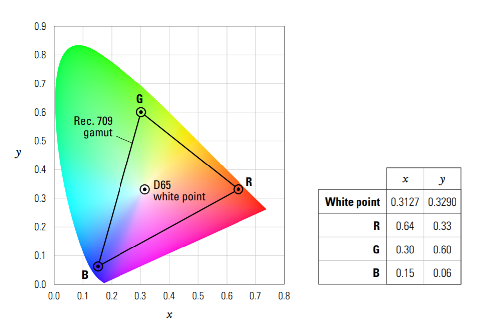
Cinematic_Color_rec709_gamut_daigram.png|500

sRGB relies on the Rec.709 primaries and White point, and thus can re-create any of the color in the above triangle (gamut).

Display-referred imagery is also the realm of ICC profiles and traditional appearance modeling techniques. If you have two different displays, with different color reproductions, you can use ICC enabled software to convert between color representations while preserving image appearance. You can also use ICC for display calibration, where libraries will compute the color transform necessary to have your display emulate an ideal calibration.

Another display-referred image specification is DCI-P3. This color space is common in digital cinema production, and is well suited to theatrical presentation. Whereas the sRGB specification uses a color encoding suited for the desktop environment, the DCI-P3 specification uses a color encoding suited for theatrical luminance levels. Another display-referred color space common in motion-picture production is X'Y'Z' (called x-prime, y-prime, z-prime ). This color space is most often utilized as the encoding actually sent to the theater in the digital cinema distribution, and is a gamma encoded version of XYZ output colorimetry⁸. See section 4.4 for further details on DCI-P3 and X'Y'Z'.

⁸ It is a mistake to colloquially refer to digital cinema s X Y Z as XYZ (omitting the primes ) - as this introduces confusion with traditional CIE XYZ. Consider referring to X Y Z as DCDM code values , as a shorter alternative.

Limitations of Display-Referred Imagery

Display-referred imagery has dynamic ranges which are inherently tied to displays. Thus, even though the real world can have enormous intensities, when working in a display-referred space values above the display-white are essentially meaningless. This mismatch between the dynamic range of the real world and the dynamic range of display-technology makes working in display-referred color spaces (even linear ones) ill suited for physically-based rendering, shading, and compositing. Yet even though working with display-referred imagery has limitations, it forms a critical component of pipelines. Thus, even in motion-picture color pipelines which work in higher dynamic range color spaces, there is always remains a portion of the pipe where display-referred, and even linearized display-referred imagery, is appropriate.

Scene-Referred Imagery

The second major image state in motion pictures imaging pipelines is that of scene-referred imagery, where the code values are proportional to real world scene measurements. The typical way to create scene-referred image is either through the characterization of a camera system, or though synthetic means (i.e., Rendering). As there is no absolute maximum White point, pixel values can be arbitrarily large within the constraints of the capture device. Scene-referred image pipelines are inherently linear, as pixel values are proportional to photons in the real world by definition.

As the real world has a very high-dynamic range, it s often useful to talk about Light in terms of stops , or doublings of light. You can compute the number of stops as the logarithm, base-2, of the luminance relative to a reference level.

r e l a t i v e e x p o s u r e = \log_{2} (\frac{l u m i n a n c e}{r e f e r e n c e l u m i n a n c e})

Relative exposure in stops, is the log, base-2, relative to some reference exposure level. Any normalization factor would suffice for relative comparisons.

Stops	Multiplication factor
-8	0.0039 (1/256)
-3	0.125 (1/8)
-2	0.25 (1/4)
-1	0.5 (1/2)
-0.5	0.707 (1/414)
0	1
+0.5	1.414
+1	2
+2	4
+3	8
+8	256

Scene-referred exposure values are often referenced in units of stops, as the range between values is rather large for directly scalar comparisons. For example, it s difficult to get an intuition for what it means to change the luminance of a pixel by a factor of 0.0039. However, it can be artistically intuitive to express that same ratio is expressed as -8 stops.

In a real scene, if you measure luminance values with a tool such as a spectroradiometer, one can observe a very wide range of values in a single scene. Pointed directly at emissive light sources, large values such as 10,000 cd/m2 are possible - and if the sun is directly visible, specular reflections may be another +6 stops over that. Even in very brightly lit scenes, dark luminance values are observed as a consequence of material properties, scene-occlusions, or a combination of the two. Very dark materials (such as charcoal) reflect a small fraction of incoming light, often in the 3-5% range. As a single number, this overall reflectivity is called albedo . Considering illumination and scene-geometry, objects will cast shadows and otherwise occlude illumination being transported around the scene. Thus in real scenes, it s often possible with complex occlusions and a wide variety of material properties to have dark values 1,000-10,000 times darker then the brightest emissive light sources.

Luminance (cd/m2)	Relative exposure	Object
1,600,000,000	23.9	Sun
23,000,000	17.8	Incandescent lamp ( lament)
10,000	6.6	White paper in the sun
8,500	6.4	HDR monitor
5,000	5.6	Blue sky
100	0	White paper in typical of ce lighting (500 lux)
50 to 500	-1.0 to 2.3	Preferred values for indoor lighting
80	-0.3	Of ce desktop sRGB display
48	-1.1	Digital Cinema Projector
1	-6.6	White paper in candle light (5 lux)
0.01	-13.3	Night vision (rods in retina)
All values are in the case of direct observation.

Luminance values in the real world span a dynamic range greater than a million to one.

It s important to observe that the real world, and consequently scene-referred imagery, does not have a maximum luminance. This differs from display-referred imagery, where it s easy to define the maximum light that a display system can emit. Considering the range of potential minimum luminance values in the real world, it is equally difficult to estimate a sensible lower limit. In common environments - physics experiments excluded - it is very hard to create a situation where there is NO light - more typical is that you just have very small positive number of photons.

When bringing scene-referred imagery into the computer it s useful to normalize the scene exposure. Even though an outdoor HDR scene may be, at an absolute level, 1000 times more luminous than the equivalent indoor scene, it is useful to have both images at equivalent overall intensities (while still preserving the relative intra-frame luminance levels). As the absolute maximum luminance is quite variable (even frame to frame), scene-referred imagery tends to be normalized with respect to an average gray level. Convention in the industry is to fix middle gray at 0.18, representing the reflectivity of an 18% gray card⁹. Observe that even when we gray-normalize the exposure of scene-linear imagery, it is expected that many portions of the scene will have luminance values >> 1.0. Note that that nothing magical happens with pixel intensities >> 1.0. Scene luminance levels represent a continuum of material properties combined with illumination; it is incorrect to assert that above a particular value (such as 1.0) would denote specularity, self-luminous objects, and/or light sources.

⁹ 18% gray is also approximately 2.5 stops below a 100% diffuse reflector.

Integer representations are not appropriate for storing high-dynamic range, scene-referred imagery due to the distribution of luminance-levels seen in real world values - even when gray normalized¹⁰. If one analyzes typical distributions of scene luminance levels, it is revealed that greater precision is required around dark values, and that decreased precision is required in highlights. For example, if one experimentally determines the smallest just noticeable difference that is suitable for recording shadow detail with adequate precision scene-linear imagery, when this same JND is used on very bright pixels, there will be far too many coding steps and bits will be wasted. Conversely, if one tailors a linear light step size to provide reasonable luminance resolution on highlights, then shadows will not have sufficient detail.

¹⁰ Integer log encodings make this feasible, of course, but will be addressed in Section 2.4.

Floating-point representations gracefully address the precision issues associated with encoding scene- linear imagery. Float representations are built from two components: the individual storage of a log exponent, and a linear fractional scaling. This hybrid log/linear coding allows for an almost ideal representation of scene-referred imagery, providing both adequate precision in the shadows and the highlights. In modern visual effects an color pipelines, OpenEXR (Appendix 4.3) is most commonly used to store floating-point imagery and helped to popularize a 16-bit half-float format. Also, while EXR popularized high dynamic range file representations in the motion-picture industry, Greg Ward made major contributions many years earlier to HDR processing and disk representations, most notably with the RGBE image format.

Characterizing Cameras

Creating scene-referred imagery is usually tackled by setting up a camera under known test conditions, and then determining how to relate the output camera RGB code values to linear light in the original scene. When going this route, its usually best to start with a camera RGB image as close to camera raw as possible, as raw encodings tend to preserve the greatest fidelity.

Even better than characterizing a camera yourself is when the manufacturer supplies this information by providing a set of curves or lookup tables to un-bake the camera-internal input transformation. In the situation where you do need to characterize a new camera (or validate that the linearization being used is accurate) the general approach is to is to set up a scene with a stable light-source, and then to do an "exposure sweep" of the camera in known increments. By changing the exposure in known f-stops, one can directly relate scene-linear exposures to camera encoded RGB code values.

Camera characterizations are often approached as channel independent mappings, using 1-D transforms. However, sometimes the camera s response is different per channel. The two common approaches to handling this are to either perform a weighted average of the channels and then use that as the basis for converting to scene-linear, or to do a different 1-D conversion for each channel. Common practice is that for systems where the channels have approximately equal response curves (most digital cameras fall into this category) to use a single mapping for all three channels. Only when capture systems have very different responses (such as film negatives) are separate curves per channel appropriate.

Channel independent mappings to scene-linear are simple, but not always sufficient. Consider two cameras from different manufacturers imaging the same scene. Even when the proper 1-D conversion to scene-linear is utilized, there are still likely to be differences in the residual color appearance due to to differing color filter / sensor technologies being utilized¹¹. These differences are often accounted for by imaging a series of color patches, and then coming up with a 3x3 matrix transform that minimizes the differences between devices. One common reference useful in such determinations is the Macbeth chart, which has standardized patches with known reflectances.

¹¹ Digital camera sensors convert incoming spectral light to RGB in a manner that does not match human color perception, for a variety of reasons related to chemistry, noise minimization, and light sensitivity.

Cinematic_Color_022.png|200

The Macbeth color checker is commonly used to validate camera characterizations; the patches have known reflectance values. Image courtesy of X-Rite.

While a full discussion of input characterization is outside the scope of this document, there are differing philosophies on what camera linearizations should aim to achieve at very darkest portions of the camera capture range. One axis of variation is to decide if the lowest camera code values represent "true black", in which the average black level is mathematically at 0.000 in scene-linear, or if instead the lowest camera code values correspond to a small but positive quantity of scene-linear light. This issue becomes more complex in the context of preserving sensor noise/film grain. If you consider capturing black in a camera system with noise, having an average value of 0.000 implies that some of the linearized noise will be small, yet positive linear light, and other parts of the noise will be small, and negative linear light. Preserving these negative linear values in such color pipelines is critical to maintaining an accurate average black level. Such challenges with negative light can be gracefully avoided by taking the alternative approach, mapping all sensor blacks to small positive values of linear light. It is important to note that the color community is continues to be religiously split on this issue. Roughly speaking, those raised on motion-picture film workflows often prefer mapping blacks to positive linear light, and those raised on video technology are most comfortable with true black linearizations¹².

¹² This author is a strong advocate of the filmic approach, mapping all blacks to positive scene-linear pixel values.

Displaying Scene-Referred Imagery

One of the complexities associated with scene-referred imagery is display reproduction. While HDR imagery is natural for processing, most displays can only reproduce a relatively low dynamic (LDR) range¹³. While at first glance it seems like a reasonable approach to directly map scene-referred linear directly to display-linear (at least for the overlapping portions of the contrast range), in practice this yields unpleasing results. See Color Management for Digital Cinema [Giorgianni 05], for further justification, and Section 3.2 for a visual example.

¹³ Displaying scene-referred imagery on high-dynamic range displays is not often encountered in practice due to the limited availability of high-dynamic range displays in theatrical environments. (In this case we are referring to the dynamic range of the maximum white, not the deepest black). This author is excitedly looking forward to the day when theatrical HDR reproduction is available.

In the color community, the processes of pleasingly reproducing high-dynamic range pixels on a low dynamic range displays is known as tone mapping, and is an active area of research. Surprisingly, many pleasing tonal renditions of high-dynamic range data use similarly shaped transforms. On first glance this may be surprising, but when one sits down and designs a tone rendering transform there are convergent processes at work corresponding to what yields a pleasing image appearance.

First, most tone renderings map a traditional scene gray exposure to a central value on the output display¹⁴. Directly mapping the remaining scene-linear image to display-linear results in an image with low apparent contrast as a consequence of display s surround viewing environment. Thus, one adds a reconstruction slope greater than 1:1 to bump the midtone contrast. Of course, with this increase in contrast the shadows and highlights are severely clipped, so a rolloff in contrast of lower than 1:1 is applied on both the high and low ends to allow for highlight and shadow detail to have smooth transitions. With this high contrast portion in the middle, and low contrast portions at the extrema, the final curve resembles an S shape as shown below.

¹⁴ Under theatrical viewing conditions, mapping middle gray (0.18) in scene-linear to approximately 10% of the maximum output luminance (in linearized display-referred space) yields pleasing results.

Scene-linear source values

An "S-shaped" curve is traditionally used to cinematically tone render scene-referred HDR colorimetry into an image suitable for output on a low dynamic range display. The input axis is log base 2 of scene-linear pixels. The output axis corresponds to code-values on a calibrated sRGB display.

The final transfer curve from scene-linear to display is shockingly consistent between technologies, with both digital and film imaging pipelines having roughly matched end to end transforms. If we characterize the film color process from negative to print, we see that it almost exactly produces this S- shaped transfer curve, which is not surprising given the pleasant tonal reproductions film offers. In traditional film imaging process, the negative stock captures a wide dynamic range (beyond the range of most modern digital cameras), and the print stock imparts a very pleasing tone mapping for reproduction on limited dynamic range devices (the theatrical print positive ). Broadly speaking, film negatives encode an HDR scene-referred image, and the print embodies a display-referred tone mapping. For those interested in further details on the high-dynamic range imaging processes implicit in the film development process, see the Ansel Adams Photography Series [Adams 84].

It s worth noting that current tone mapping research often utilizes spatially varying color correction operators, referred to as local tone mapping, as the local image statistics are taken into account when computing the color transform. While this research is very promising, and may impact motion picture production at some point in the future, most motion-picture color management approaches currently utilize a global tone mapping operator; the underlying assumption that each pixel is treated independently of its neighboring values. However, much of the current look of spatially varying tone mapping operators are currently achieved cinematically in alternate ways. For example, local tone mapping operators often accentuate high-frequency detail in shadow areas; detail which would have otherwise been visually masked. In the cinematic world, this is often accomplished directly on-set by the cinematographer when setting up the actual lighting, or as an explicit, spatially varying artistic correction during the digital intermediate (DI) process.

To summarize, we strongly advise against directly mapping high-dynamic range scene-referred data to the display. A tone rendering is required, and there is great historical precedence for using a global S-Shaped operator. HDR scene-acquisition accurately records a wide range of scene-luminance value, and with a proper tone mapping operator, much of this range can be visually preserved during reproduction on low-dynamic range devices.

Please refer to Section 3.2 for a visual comparison between an S-shaped tone mapping operator versus a simple gamma transform.

Consequences of Scene-Referred Imagery

Working with the dynamic ranges typical of scene-referred imagery positively impacts almost every area of the computer graphics pipeline, particularly when the goal is physical realism. In Rendering and shading, scene-referred imagery naturally allows for the use of physically-based shading models and Global Illumination. In compositing, physically-plausible dynamic ranges allow for realistic synthetic camera effects, particularly as related to filtering operations, defocus, motion-blur, and anti-aliasing. Section 3 further details how scene-linear workflows impact specific portions of the motion-picture color pipeline.

Unfortunately, scene-referred imagery also presents some challenges. Filtering, anti-aliasing, and reconstruction kernels which make use of negative-lobed filters are more susceptible to ringing when applied to HDR imagery. While high-dynamic range data isn't the root cause of the ringing, it certainly exacerbates the issue. Another pitfall of working with HDR imagery is that storage requirements are increased. In a low dynamic range workflow 8-bit pixel representations per component are sensible, while in HDR workflows 16-bits per component is usually a minimum. There are further issues when compositing in scene-linear, as many of the classic common compositing tricks rely on assumptions which do not hold in floating point. Section 3 outlines potential solutions to many of these issues.

A Plea for Precise Terminology

Both the motion-picture and computer graphics communities are far too casual about using the word linear to reference both scene-referred and display-referred linear imagery ¹⁵. We highly encourage both communities to set a positive example, and to always distinguish between these two image states even in casual conversation.

¹⁵We have even witnessed members of the community - who shall remain nameless - reference Rec. 709 video imagery as linear . Such statements should be confined to the realm of nightmares.

To clarify, are you referencing the linear light as emitted by a display? Did you use the word gamma? Are there scary consequences to your imagery going above 1.0? If so, please use the term display-linear.

Are you referencing high-dynamic range imagery? Is your middle gray at 0.18? Are you talking about light in terms of stops ? Does 1.0 have no particular consequence in your pipeline? If so, please use the term scene-linear. Finally, for those using scene-linear workflows remember to use a viewing transform that goes beyond a simple gamma model. Friends don t let friends view scene-linear imagery without an S-shaped view transform.

Color Correction, Color Space, and Log

It is sometimes necessary to encode high-dynamic range, scene-referred color spaces with integer representations. For example, digital motion picture cameras often record to 10-bit integer media (such as HDCAM SR or DPX files). As noted earlier, if a camera manufacturer were to store a linear integer encoding of scene-referred imagery, the process would introduce a substantial amount of quantization. It turns out that using a logarithmic log integer encoding allows for most of the benefits of floating point representations, without actually requiring float-point storage media. In logarithmic encodings, successive code values in the integer log space map to multiplicative values in linear space. Put more intuitively, this is analogous to converting each pixel to a representation of the number of stops above or below a reference level, and then storing an integer representation of this quantity.

As log images represent a very large dynamic range in their coding space, most midtone pixels reside in the middle portion of the coding space. Thus, if you directly display a log image on an sRGB monitor it appears low contrast (as seen below).

Cinematic_Color_023.jpeg|500

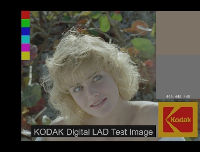
This image is using an integer logarithmic encoding to represent a high dynamic range of scene intensities, and thus appears low contrast when mapped to the display. This image is colloquially known as Marci, and is a common reference image in theatrical exhibition. This image originated as a scan of a film negative (courtesy Kodak Corporation), and can be downloaded from their website.

Not all log spaces are equal. Most camera manufacturers customize a log encoding equation to optimize the usage of code values based on the camera s dynamic range, noise characteristics, and clipping behavior. Examples of different log spaces include Sony S-Log, RED s REDLog, Arri LogC, and the classic Cineon¹⁶. Care must be taken during image handling to determine which log space is associated with imagery, and to use the proper linearization. If this metadata is lost, it is often challenging to determine after the fact which log flavor was using in encoding.

¹⁶ The Cineon log encoding differs from digital motion-picture camera log encodings in that Cineon is a logarithmic encoding of the the actual optical density of the film negative.

Motion-Picture Color Management

A Color Pipeline is the set of all color transformations used during a motion-picture production. In a simplified computer graphics pipeline (below), we consider processes such as texture painting, matte painting, on-set lighting capture, traditional motion-picture camera inputs, lighting, Rendering, compositing, and digital intermediate (DI). In a properly color-managed pipeline, the color encodings are well defined at all stages of processing.

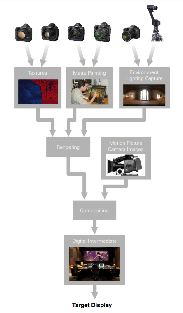
Cinematic_Color_color_management_scheme.png|500

A well-defined computer-graphics color pipeline rigorously manages the both color transformations applied at each stage of the process, in addition to the transforms required for accurate image preview.

We define the color pipeline by carefully tracking the color encodings (color space) for all image inputs, image outputs, and intermediate representations. We also rigorously define the transforms used to convert between color spaces.

Visual Effects Color Pipelines

The traditional visual effects color pipeline is based around the core principle of doing no harm to the plate, to allow for the seamless intercutting of vfx and non-vfx shots. Plate photography is brought into the pipeline in whatever color space is delivered (camera log, commonly), and then typically converted to scene-linear using an invertible transform. Often a pure 1-D camera to linear transform is used, though sometimes the linearization is augmented with a matrix transformation. For visualization, a 3D-LUT is used which emulates the eventual output processing, which may either be a print film emulation or a similar S-shaped transformation. During the visual effects process, the display transform is never baked into the imagery except for throw-away deliveries such as editorial output or rough preview screenings. The delivery to DI is expected to be the highest-fidelity representation of the original photography.

Animated Feature Color Pipelines

In animated feature color pipelines, all imagery is generated synthetically within the computer. Thus, plate invertibility is a non-issue and far more latitude is allowed in the selection of viewing transforms. Nonetheless, despite such freedoms it is often preferable to carry over those aspects of the traditional film workflow which are beneficial even in a fully-CG context. We thus advocate thinking of an animated feature as creating a virtual movie-set within the computer, complete with a virtual camera, virtual negative stock, and virtual print stock. Of course, while these virtual color transforms can be inspired by real-world counterparts, it is generally preferable to use idealizing simplifications which do not delve into the colorimetric peculiarities inherent to physical imaging workflows.

Roughly speaking, physically-inspired animated feature color pipelines require two unique transforms: a conversion from scene-linear to the log-integer encoding space suitable for DI handoff (the virtual negative) and a viewing transform used for viewing the virtual negative (the virtual print). The virtual negative transform is baked into the imagery prior to DI, and the virtual print transform is baked into the imagery post-DI. Typically these transforms are defined as 1-D curves (equal per channel), and may include matrixing. Complicated 3-D LUTs, common in VFX workflows, are typically avoided except during print-film theatrical release (and creative uses of trim passes during DI may totally eliminate the need for such an inverse film print 3D-LUT ).

Animated-feature color workflows have historically relied upon a single-step viewing transform, which directly converts from linear to the display, often using a gamma transform¹⁷. However, physically inspired animated-feature color workflows (which separate the negative vs. print transform) are becoming increasingly preferred due to the ease of working with HDR rendering spaces and the robust hand-off to DI.

¹⁷ This viewing transform should set off warning flags in the reader that such pipelines are really operating in a display-linear, rather than a scene-linear, rendering space. Look back upon Section 2.3, "A Plea For Precise Terminology , and section 2.3, for details.

Digital Intermediate, Mastering, and Delivery

Digital intermediate (DI) is the process where the entire motion-picture is loaded into a dedicated hardware device, for the purpose of color-correcting in an environment that exactly mirrors the final exhibition (i.e., in a theater). Viewed in this final environment, DI is where per-shot color corrections are added, and the visual look of the film is finalized. DI is also referred to as color timing, or grading. The final step of baking in view transforms specific to an output device, and final color correction, is known as mastering.

Cinematic_Color_048.png|500

Locking down the eventual DI viewing transform(s) early on in the critical first step in crafting cinematic color pipelines, as it pins down every other part of the process. The remainder of the pipeline essentially relies on visualizations that are created by working backwards from this step.

Digital intermediate is done in a viewing environment that exactly mirrors the final exhibition. If you are mastering for digital cinema, the DI must be done in an equivalent theatrical setting with matched digital projection. If you are mastering for home theater, you should be mastering in an equivalent idealized home environment¹⁸. If you are mastering for film release, you typically use a theatrical environment with a digital projector, with a film emulation 3D-LUT made in conjunction with the print house to confirm a visual match. Digital intermediate (and mastering) typically have very tight tolerances on calibration, as the decisions made in this process are the last time image color appearance is tweaked.

¹⁸ Most common mastering environments have rigorous specification, often defined by SMPTE. These lock down expectations for colorimetry, device calibration, and even environmental concerns such as surround luminance.

Examples of popular commercial DI systems include Lustre, DaVinci, Baselight, NuCoda, etc. Companies that historically have historically done DI include Deluxe and Technicolor.

Color Correction and Working Space

There are two main approaches to handing color in digital intermediate. The first video-centric approach is where display-referred imagery is loaded into the DI; no viewing transform is necessary. The display-referred frame buffer is directly manipulated in the color corrector (akin to a motion-picture version of Photoshop). In the second film-centric approach, scene-referred imagery is loaded into the machine and a viewing transform (3D-LUT) is required to create the final the color appearance. The color correction manipulates the underlying scene-referred representation, but all color judgements are made previewing through the display transform.

The advantage of the video approach is one of process simplicity. When color correcting pre-rendered imagery, a relatively modest amount of color correction can be applied without introducing artifacts in the imagery. The downside to this approach is that much of the detail in the original imagery is lost when pre-baking in the view transform. Indeed, in some implementations this baking in of the view transform may even be internal to the camera (or in animated features, inside the Renderer). For example, if a shot was originally overexposed, a sensible color correction is to darken the image. However, it is likely that in the overexposed image that large portions of the image was clipped to a constant maximum value, and no possible correction can bring back this lost detail.

In the "filmic" approach, working with a scene-referred imagery, a high-fidelity representation of the full dynamic range from the original camera is loaded into the color corrector. Camera raw imagery is directly graded on rare occasion, but more commonly a camera-specific integer log encoding is utilized. In the future, DI systems that load floating-point scene-referred imagery will become increasingly common, but for now log DPX files are the norm. For viewing, an S-shaped tone curve is utilized; crafted to precisely emulate the appearance on the reference output display device. For example, on a motion-picture that intends to have a film print theatrical distribution, it is appropriate to select a 3D-LUT for viewing which emulates the specific development and print process. If this film is to also be distributed digitally, this specific print film emulation will be baked into the imagery, post DI, but prior to digital distribution. Of course, if the production will only be distributed digitally there is far more latitude in selecting a viewing transform. In both cases, the appearance of the imagery in DI is modified by color correcting the image in the scene-linear (or log encoded) color space, and making visual decisions based on the appearance post view transform.

Going back to our over-exposed example, remember that more of the dynamic range from the original camera capture is preserved when using a scene-referred approach. Thus, when we change the exposure on our log data we may expose new details which had not previously been visible (no clipping has occurred). In terms of classic film production processes, as more data was captured on the negative, we have a wide latitude of possible print exposures over which a high print fidelity is maintained. This allows color correction in log DI to be very high fidelity; most modest corrections do not drive the image to flat black or flat white.

DPX is commonly used as a log delivery format to digital intermediate, and both 10-bit and 16-bit versions are common-place. For grainy material, 10-bits is often sufficient, but 16-bit is becoming increasingly common for low-noise computer-generated imagery¹⁹. In the case of passing true scene- linear renders directly to DI, 16-bit floating point (EXR) is preferable. 16-bit integer linear representations are not recommended.!

¹⁹ This is not to imply that computer-generated imagery is inherently low noise. Indeed, with modern Rendering techniques such as Global Illumination often the alternative is true (live action being less noisy than CG).

An original log film plate (top-left) is loaded into the DI color corrector. When viewed with a film emulation table (top-right), the appearance is predictive of the final output with a default exposure. If we were to lower the exposure using an additive offset in log-space (lower-left), new details in the flame highlights are revealed. When a similar correction is applied to a color-corrector working in a display- referred space (lower-right), this detail is lost. Imagery from Spider-Man Courtesy of Columbia Pictures. ' 2002 Columbia Pictures Industries, Inc. All rights reserved.

In scene-linear, a gain operation is typically used to change the color balance and scene exposure. In log space, this roughly corresponds to offsets. If a mathematically exact log is used, they are in fact identical, though most manufacturers tweak the log encodings as previously mentioned. Log offset color corrections (per color channel) are ubiquitous in motion-picture industry color correction; often referred to as the primary grade or one-light. Theatrical fades to black have a very particular appearance to them, which is a direct consequence of the fade applying in log space, as viewed through the traditional S-shaped film emulation. Fade to blacks applied as gain operations in scene-linear have a roughly similar visual appearance, with specular highlights lingering on screen well beyond midtones.

Artistically, the DI process can be segmented into a per-shot correction that neutralizes shot to shot color variation, and then a secondary process that crafts the overall artistic look of the film. It is common for the DI house, if an initial grade happens early enough, to communicate to the VFX houses the looks being used. This often is send as a CDL, or a 3D-LUT, per shot, and does not have the viewing transform baked into it. It is also important to communicate the color space that the color corrections have been applied in. Most often, the color correction DI color space is the same as the visual effects delivery format. The advantage of working with this data downstream is that for computer-generated imagery, you have have a better preview of the eventual appearance of the theatrical release.

Trim Passes and Mastering

It is common in DI to create masters for multiple output devices. For example, on major motion- pictures one may be expected to deliver masters for digital projectional, film release, home theater (in both HD and standard def), at a mix of 2-D and 3-D. The general approach is to identify one output process as the gold standard, and to spend the majority of the artistic time correcting the images to look perfect on that device. In our experience, the theatrical digital projection is most often the appropriate master to treat as reference. The director, producers, and other creatives will be present at this process. Once the main color grade is complete, additional masters are handled as trim passes atop the main output. Trim passes are most often implemented as additional color correction layers added atop primary corrections, and only utilize minor corrections such as contrast, brightness, and saturation. The display transform baked into each master is device-specific; a different view transform tailored to each output device is a necessity. Creatives do not need to be present during the creation of trim passes, as the colorist already familiar with the final look of the material, and has a known reference to use as a color appearance target.

The motion-picture viewing environment greatly impacts color appearance. Theatrical viewing environments typically have dark surround and a relatively low screen luminance (48 cd/m2 is common). In the home theater, a dim surround is likely and a brighter screen luminance of 80 cd/m2 is typical. In a desktop/office setting, a bright surround is likely. Thus, if you display the same image in each environment, the appearances will be very different, most specifically the perceived image contrast and colorfulness. Color appearance models may be used to attempt to correct for these settings, but trim passes with a human in the loop typically yield far higher fidelity results.

When mastering for stereoscopic 3-D, an additional 3-D specific trim pass is a necessity. Due to the additional optics necessary to create the stereo image pair (additional filters in the projector, glasses on the audience) the projected stereo image is usually far lower luminance than traditional 2-D theatrical projection. As lower luminance images tend to appear less colorful, the trim passes for stereo masters typically boost both the saturation and contrast relative to the 2-D master.

Lighting, Rendering, Shading

The stages of Rendering, lighting, and shading most closely approximate physical realism when performed in a high-dynamic range, scene-linear color space. Ideally, no color space conversions should be required during the execution of the render, as all input assets such as textures, plate re-projections, and skydomes, can be linearized beforehand. Image viewing of scene-linear data is typically handled by converting to the color space being delivered to digital intermediate (commonly a log color space), and then applying the view transform suitable for the specified display. For convenience, these transforms are typically baked into a single 3D-LUT, though care must be taken to assure the LUT has suitable fidelity over an appropriate HDR domain. As mentioned earlier, you must use a viewing transform when viewing HDR scene-linear data.

Cinematic_Color_053.png|500

In this raw visualization of a high dynamic range, scene-linear render, values greater than 1.0 are clipped when sent to the display (though present in the underlying image file).

Cinematic_Color_054.png|500

Using a naive gamma 2.2 visualization (directly mapping scene-linear to display-linear), results in an image with low apparent contrast and poor highlight rendition (observe clipping on the table.)

Cinematic_Color_055.png|500

Using an S-shaped tone curve to visualize the scene-linear render yields a pleasing appearance of contrast, with well balanced highlight and shadow details.

Renders by Sony Pictures Imageworks, available for download at opencolorio.org. Images from Cloudy With a Chance Of Meatballs Courtesy of Sony Pictures Animation. ' 2009 Sony Pictures Animation Inc. All rights reserved.

Why is scene-linear preferred for lighting? First, the render itself benefits. Physically plausible light transport Renderer mechanisms such as Global Illumination yield natural results when given scenes with high dynamic ranges. Physically-based specular models, combined with area lights, produce physically plausible results with high-dynamic range data. Rendering in scene-linear also allows lights and material components to be re-balanced post-render, with results that track identically to if the original render had been tweaked. Storing rendered images in a floating-point container is most common to preserve maximum image fidelity; the OpenEXR format (section 4.1) is most common in VFX and animation.

One issue to watch out for with high dynamic range renders is render noise. When scene textures (such as skydomes) contain emissive specular areas that substantially contribute to the scene illumination (RGB >> 1.0), care must be taken in terms of sampling or noise is likely. Modern Rendering enhancements such as multi-importance sampling (MIS) are useful to mitigate such issues. Even still, it is common to paint out very compact and/or bright light sources (such as the sun) from skydomes, and then to add them back into the scene as native Renderer lights to allow for both lower-noise sampling and often greater artistic control.

Light shaders also benefit from working with scene-referred linear, specifically in the area of light falloff. In the past, the default mode of working with lights in computer-graphics was to not use falloff. However, when combined with physically-based shading models, using an r2 light falloff behaves naturally. If one tries to shoehorn in realistic lighting falloff models into lower dynamic range spaces (such as display-referred linear), it s very difficult to avoid clipping. On the downside, one consequence of working with natural light falloff is that it s often required to have very high light intensity values. It is therefore common to express light intensity in user interfaces in terms of stops, as it s much friendlier to the artist to present an interface value of +20 stops, compared to a RGB value of 1048576.0 .

Anti-aliasing operations also benefit from scene-linear, though one must be more careful with Renderer reconstruction filters. Negatively lobed filters such as Catmull-Rom have an increased tendency to exhibit ringing due to the extra dynamic range. This is a particular problem on elements lit with very bright rim lights, as this creates bright specular highlights directly in contact with edges. There are two common approaches to working around such filtering issues. First, very bright specular samples can be rolled-off such that these samples do not contribute such large amounts of energy. However, this throws out much of the visually significant appearance which adds so much to the realism. Another approach is that the extra energy can be spread amongst neighboring pixels such that the specular hits show an effect analogous to camera flare. Both of these effects can be implemented either during compositing or internal to the Renderer; the advantage of the latter is the processing can work on the sub-pixel level for higher quality anti-aliasing.

HDR Environment Captures

HDR captures are increasingly being used to capture onset lighting. Historically, the classic technique to capture spherical environment maps to was photograph a chrome ball, as first pioneered by Gene Miller²⁰. Recent advances in hardware now allow for directly capturing the scene-illumination, either with a multi-exposure fisheye camera or with dedicated hardware. One recent extension to this methodology is to capture the scene from multiple heights and/or locations, which through triangulation allows for plausible energy estimations of the scene-lighting. Such energy estimates allow for physically plausible rendering of local illumination effects, which contrasts with traditional skydome rendering approaches which assumes infinitely distant lights.

²⁰ See [Debevec 06] for a fascinating retrospective on the history of environment mapping.

Care must be taken when calibrating HDR lighting acquisitions to account for colorimetry, linearity, and white balance, or the resulting lighting data may not integrate into the computer-generated environments. Adding a diffuse sphere and other reference materials during scene capture is useful in validating the lighting reconstruction later on.

Compositing

Compositing is the process where live action plates are merged with computer-generated imagery. Image processing in both scene-linear and logarithmic encoding spaces are both useful, though scene- linear is increasingly the default. As in lighting, image display typically leverages viewing transforms that emulate the eventual DI process. Examples of commercially available compositing applications include Nuke, After Effects, Fusion, and Flame.

In feature film visual effects, plates (live action photography) are typically represented on disk as a log encoding of the linear camera data, often as DPX files. Frames when brought into the compositing package are typically converted to scene-linear on input, and then converted back to the original color space on output. End to end, the compositing process represents a no-op, and typically aims for perfect invertibility in color processing. Such a behavior is absolutely critical, as typically not all the shots will go through the VFX workflow, and VFX processed shots must seamlessly intercut with the remainder of the motion-picture.

The benefits of scene-linear compositing are numerous; similar to the benefits found in Rendering, shading, and lighting. All operations which blend energy with spatially neighboring pixels (motion blur, defocus, image distortion, resizing, etc) have more physically plausible (aka realistic) results by default. Anti-aliasing works better, light mixing preserves the appearance of the original renders and most importantly, even simple compositing operations such as over produce more realistic results, particularly on semi-transparent elements (hair, volumetrics, fx elements, etc).

Cinematic_Color_056.jpeg|500

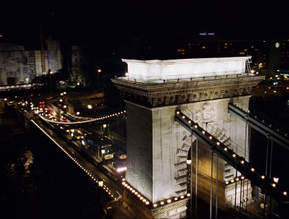
This image helps illustrate the energy implications of using different linearization philosophies. Pay particular attention to the appearance of the string of lights on the top of the bridge span. How much energy is represented in those pixels?

Cinematic_Color_057.jpeg|500

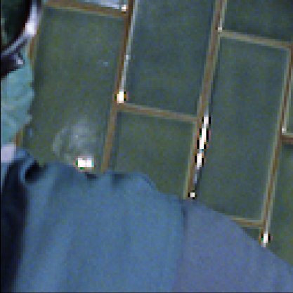
Applying a defocus in scene-linear reveals a bokeh effect on each of the bridge span lights, mimicking the visual look of having performed this defocus during camera acquisition. This is because the pixel values are proportional to light in the original scene, and thus specular pixels have sufficient energy to remain visible when blended with their neighbors. Other energy effects such as motion-blur achieve similar improvements in realism from working in a scene-linear space.

Cinematic_Color_058.jpeg|500

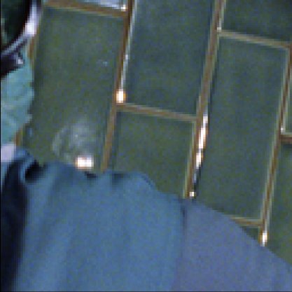
Applying the same defocus in display-linear tends to de-emphasize the specular highlights. This is because even though the operation is being applied in linear, post-display transform, the highlights have already been tone rendered for a lower dynamic range display and thus do not have physically- plausible amounts of energy.

Scene-Linear Compositing Challenges

There are some challenges with working with high-dynamic ranges in compositing. First, filtering operators that use sharp, negative lobed kernels (such as lanczos, keys, sinc,) are very susceptible to ringing (negative values around highlights) . While interpolatory filters such as box, gaussian, bilinear, and bicubic cannot cause this artifact, they do introduce softening. For cases where sharp filtering is required (lens distortions, resizing, and other spatial warping techniques) a variety of approaches are useful to mitigate such HDR artifacts.

The simplest approach to mitigating overshoot/undershoot artifacts is to rolloff the highlights, process the image, and then unroll the highlights back. While this does not not preserve highlight energy (it has the net effect of reducing specular intensity), the results are visually pleasing and is suitable for processing images with alpha. Another approach to HDR filtering is to apply a simple camera flare model, where very bright highlights share their energy with neighboring pixels. Finally, for images without alpha, converting to log, filtering, and converting back will greatly reduce the visual impact of overshoot and undershoot. Though log-space processing results in a gross distortion of energy, for conversions which are approximately 1:1 (such as lens distortion effects for plates) this works well.

Cinematic_Color_059.jpeg|500

Applying negative-lobed filter kernels to high-dynamic range images (in this case a lanczos3 resize) may cause visually-significant ringing artifacts. Observe the black silhouettes around the sharp specular highlights.

Cinematic_Color_060.jpeg|500

Ringing artifacts may be avoided when using sharp filters on HDR imagery by processing in alternate color representations (such as log), using energy-rolloff approaches, or by pre-flaring highlight regions. This image demonstrates the results of the roll-off technique.

Another challenge in working with scene-linear data in compositing is that tricks often relied upon in integer compositing may not be effective when applied to floating-point imagery. For example, the screen operator (which remains effective when applied to matte passes), is sometimes used on RGB data to emulate a partial add . As the screen operator is ill-defined above 1.0, when applied to HDR data unexpected results will be common. Some compositing packages swap out screen for max when either input is outside of [0.0, 1.0], but this is primarily to prevent artifacts and is not artistically helpful. Alternative partial add maths such as hypotenuse are useful, but do not exactly replicate the original intent of screen. Another related issue to beware of when compositing is that when combining HDR image, alphas must not go outside the range of [0,1]. While it is entirely reasonable for the RGB channels to have any values (even negative in certain cases!) the compositing operators, such as over, produce totally invalid results on non [0,1] alphas.

One subtlety of working with floating point imagery is that artists must become familiar with some of the corner cases in floating-point representations: NaNs and Infs. For example, if one divides by very small values (such as during unpremultiplication) it is possible to drive a color value up high enough to generate infinity. NaNs are also frequent, and may be introduced during shading (inside the Renderer), or during divide by zero operations. Both nans and inf can cause issues in compositing if not detected and cleaned, as most image processing algorithms are not robust to their presence and generally fail in unexpected ways.

Working with Log Imagery

Despite HDR having benefits in many compositing operators, there are just some cases even in modern compositing workflows where log-like spaces are still useful. For example, manipulating contrast of HDR images is non-trivial. Contrast is typically describes as a color correction which makes the shadows darker, and the highlights brighter, centered around some pivot. In unconstrained floating-point spaces, if you use a linear + offset contrast operator (mx+b), it is difficult to choose offsets that do not drive pixels negative. And the alternative, a gamma function (exponentiation), has the potential to drive highlights to disturbingly large values. This is one of the cases where a conversion to a log-like space is very helpful. In log space, both the linear and gamma contrast operators have reasonable performance. This is one of the reasons that DI color work is often preferred to work in log-like spaces. Other operations which are useful to perform in log are grain matching, pulling keys, and many spatial distortion operators. But be careful when using log color spaces in compositing, as not all log

transforms preserve the full range of scene-linear code values. Many such conversions clip values above certain highlight color, below a certain shadow color, and most often clip all negative values. Finally, compositing must also generate plates for DI that hold up under a variety of color corrections. See the section on Critical inspection of imagery for further details.

Plate Timing / Neutralization

When working with plate photography it is often useful to come up with simple color corrections for each plate to neutralize the lighting across a sequence. During the shoot, there will inevitably be color drift across the shots (such as the sun moving behind a cloud, the lights moved to different locations, etc). Using neutralized plates in lighting and compositing leads to nice gains in efficiency as light rigs and sequence standards track better. In most workflows the plate neutralization is done at the top of the compositing graph, the rendered neutral elements are composited in, and then before the file is written out the neutralization is undone. This approach is often called reverse out, and its advantage is that the output delivery is consistent with the input plate, independent of the color neutralization process. Color corrections used for plate neutralization must be reversible, and as such are typically handled as either simple offsets in camera log space, or as simple gains in linear. More complex operations such as contrast, saturation, etc. are usually avoided as these type of corrections break the linearity of the plate and will likely make compositing more difficult (presuming the linearization was handled done to begin with).

It is important to draw a distinction between timing number necessary for plate neutralizations, and the potentially more sophisticated looks that are crafted in the DI. At DI, the full suite of color correction operators can be used (contrast, keys, primaries, secondaries, etc), as there is no need to ever invert this process. However, the color neutralization numbers needed for lighting and compositing must be invertible, and as such are typically limited to a simple color balance adjustments. Beware that if you bake in the neutralized color correction, you must preserve this extended range throughout the downstream compositing and delivery processes. I.e., if your compositing package uses a log-convert on input, and then you color timing, you must confirm that downstream log-converts on the neutral graded imagery are not clamping either the high or low end.

Premultiplication

Premultiplication gets an unwarranted bad rap, as the name implies that one starts with an RGB color, adds the concept of transparency, and then premultiplies by it. This isn t actually true. Premultiplied RGB is the natural representation for color and transparency and is the native output of renderers. A nice mental model for premultiplied RGBA is that the RGB channels represent how much light is emitted from within the region of the pixel, and alpha represents how much a pixel blocks light behind it. As alpha represents the fraction of occlusion, to maintain physical correctness alpha values must be between 0 and 1. RGB channels have no such constraints, and can range from -infinity to infinity.

Furthermore, there is absolutely no issue with RGBs greater than alpha (a common misconception). Even when alpha is zero, a positive RGB is completely reasonable - corresponding to light being emitted from a pixel without occluding anything behind it. Indeed, this situation is common in emissive FX renders such as fire.

So how should we interpret unpremultiplied RGBA? Unpremultiplied RGBA is most easily understood as, If* this pixel were fully opaque, how much light would have been emitted? This representation is certainly useful in specific compositing contexts (such as when pulling luma keys from CG elements), but as converting to unpremultiplied RGBA is a lossy approximation it s prudent to only do the conversion when absolutely necessary.

For additional information on premultiplied vs. unpremultiplied RGBA representations, see [Duff 84] and [Blinn 98].

Texture and Matte Painting

Texture painting and matte painting present a color pipeline challenge. Ideally, one could directly paint in a scene-linear space and use appropriate visualizations to get realistic previews of the eventual render appearance. However, the majority of texture painting applications work most intuitively in display- referred color spaces, where the painted image is directly displayed on the screen. Furthermore, texture reference is often acquired as display-referred imagery (such as the JPG/TIFF output from a digital camera); scene-linear texture reference is only available in rare situations.

Cinematic_Color_061.jpeg|500

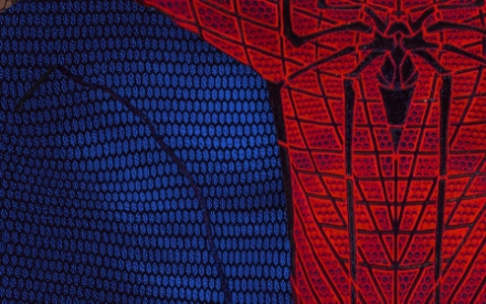
This color map represents the color modulation of the diffuse component of a surface shader, and is painted in a display-referred space. When converted to linear (prior to mipmapping) the resulting color values range between [0,1] and are representative of physically-plausible surface albedos.

Thus, a common solution is to utilize an inverse tone rendering, to back convert display-referred imagery to a hypothetical scene-referred space. Conceptually, the texture artist is painting the tone rendered appearance of the texture, not the texture itself. There are a few challenges with this conversion from display-referred to scene-referred space. First, the tone rendering may not be invertible, particularly when filmic 3D-LUTs are used for image preview. Second, traditional s-shaped tone renderings have very horizontal portions of the curve, which when inverted result in very steeply sloped transfer functions. This steep contrast has the effect of amplifying small changes in input code values. For example, a steep inverse could result in the situation where a single code value change in a painted texture could correspond to a delta of a stop or more of scene-linear light. This sensitivity is very challenging for artists to work with.

A common solution to both of these issues is to be a bit more modest in our goal of perfectly inverting the display transform. Simplifying the problem, we can instead aim to create an approximate 1-D inverse, tuned to be well behaved both in terms of color performance and dynamic range. Of course, as a consequence of this simplification the texture painting is not be truly WYSIWYG. Thus, a residual "difference visualization" 3D-LUT is crafted for accurate color preview in the texture painting tool.

It is often useful to consider matte painting and texture painting as two different color transforms. In matte painting, it is very common for the artist to want to paint values which will eventually utilize the full scene-linear dynamic range, even when working in a display-referred space. Thus, an inversion which allows for the creation of bright specular values is preferable. In such cases, it is often convenient to provide a visual preview both at a normal exposure, as well as a few stops darker, to let the artist have a good feel for the dynamic range in their plate.

In texture painting, the artist often paints color maps which when linearized will control material color reflectivity, as an input to physically-based shading. In these situations, linear data from [0,1], representing physically plausible surface albedos, is required and necessitates a color transform that gracefully handles these limits. One must also distinguish painted color maps from data maps (bump maps, normal maps, iso maps, control maps, etc), which should not be processed colorimetrically.

Cinematic_Color_062.jpeg|500

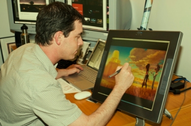
Matte painters typically prefer to paint in a display-referred color space for convenience. But as renders are natively in scene-linear, an inverse display transform is used to synthesize plausible scene-linear colors prior to rendering.

When texture acquisition is done in a controlled environment, it s possible to create scene-linear texture conversions leveraging camera raw workflows. Command-line utilities such as dcraw allow color pipelines which capture a reasonable linear representation of surface color. The use of polarizing filters and softbox lighting during acquisition further allows for increased reference texture fidelity.

Another axis of variation in texturing is when to perform the conversion to scene-linear. The approach we advocate is to linearize prior to mipmap texture generation. The primary advantage of this approach is that scene-linear energy is preserved through all the mipmap levels, allowing for the highest fidelity sampling and fewest color space related artifacts. Further, disallowing color space conversions at shading time prevents shaders from doing evil (non-linear) color math. The disadvantage is that the storage requirements for linearized data are potentially increased. I.e., even if a texture is painted at 8-bits of precision in a display-referred space, after linearization to scene-linear increased bit-depths are required. When dealing with 16-bit painted textures, this is less of a concern.

Critical Inspection of Imagery

One unfortunate reality in film production is that the typical artist display is not as high fidelity as the eventual theatrical viewing environment; most often the theatrical audience will see more color detail than the original artist. Furthermore, while artists typically craft imagery assuming a particular viewing exposure, during DI is possible that the imagery will be stylistically color corrected in unanticipated direction²¹. It is therefore critical to inspect the imagery under a variety of "worst-case" color corrections, to make sure the computer-generated imagery is as robust as possible.

²¹ Murphy s Law is a good first-order approximation of DI color correction.

At a minimum, artists working in scene-linear (namely the lighter and compositor) should aspire to view their imagery at a range of exposures as part of their regular production workflow. This enables artists to have a true sense of the dynamic range in their imagery, and to match computer-generated elements with similar precision. In compositing, it is also expedient to convert the imagery to the color space, quantization, and clamping that will be delivered to DI, to test how the imagery holds up to drastic color grades. We recommend playing with substantial log space offsets, as well as contrast and saturation boosts, to validate that all portions of the imagery track in a consistent manner. This is particularly important to match across shots and sequences, for it s all too easy to make individual shots that are self consistent, yet fall apart when viewed side to side. Most critical is the inspection of shadow detail.

"Stopping up" the final composites, shadows should have a consistent color and density both inter-shot and intra-shot, flat-black portions of the image should be avoided - lest they reappear in DI - and grain/ noise must match between the live action and the computer-generated imagery. Inspecting highlights, one should confirm that their intensity, color, sharpness, and flare appearance are similarly consistent.

Histograms are a useful tool when analyzing image fidelity, and often help forensically track down if post-processing has been applied to an image. For example, log frames from certain motion-picture cameras often do not make full use of the integer coding space. This can be detected in the histogram, and is helpful to track down an image color space when the original is unknown. The application of sharpening filters (detectable from their residual undershoot and overshoot) can also be observed in the histograms. It is possible to detect if image quantization has occurred, appearing as tell-tale comb-like peaks and valleys in the histogram. We have found that it is also a valuable tool to leverage histograms computed on HSV-transformed imagery as a final quality-check.

There are other image artifacts, such as aliasing, that are best inspected on moving imagery. For example, the use of interpolatory filters (such as nearest-neighbor or bilinear interpolation) are often unobjectionable on still imagery, yet artifact-inducing on slowly animating transforms (particularly near horizontal lines). Always be on the lookout for moire patterns and other high-frequency artifacts, particularly when such filters have been applied to imagery with high frequency details (examples: cloth/ wave patterns). If all digital imagery were ideally sampled, this would not be an issue. However, camera manufacturers have a tendency to bias imagery to be overly-sharp²² and motion transformations accentuate such artifacts.

²² Digital-motion picture camera manufacturers strenuously avoid soft reconstructions, Nyquist be damned. Always be skeptical of camera resolution claims without accompanying resolution charts.

For stereo deliveries, it s critical to quality check both eyes individually, as well as together in a proper stereo viewing environment. There are many stereo artifacts which are only visible on true 3-D displays, and catching these early on is most cost-effective.

ACES

The Academy of Motion Picture Arts & Science has proposed a unification of scene-linear floating-point workflows, which adheres to many of the approaches outlined in this document. If successful, the ACES project will allow for the unambiguous interchange of floating point imagery. At its core is the Academy Color Encoding Space, called ACES for short. This color space is a high-dynamic range, scene-linear space, with middle gray pegged to 0.18, and a very wide Color gamut. When stored on disk, ACES files are stored in a constrained version of the OpenEXR format.

The ACES workflow defines scene-referred working space, and a reference viewing transform, in an attempt to standardize float-linear interchange in the motion-picture industry.

The Academy also defines the viewing transform necessary for viewing ACES files. The view transform is conceptually segmented into two portions. First, the Reference Rendering Transform (RRT) applies a local contrast boost and tone-renders scene-linear imagery to display linear. Then, a second portion of

the view transform called the Output Device Transform (ODT) is used to provide gamut mapping and further tone mapping to the target output device. The RRT portion is constant across all displays, but the ODT varies from output display device to output display device. ODTs are provided for common display specifications such as sRGB, Rec. 709, DCI-P3, X Y Z , etc.

On the input side, a series of published input device transforms (IDTs) for specific image acquisition devices convert input colorimetry to scene-linear (ACES). Film scans are a special case, where the academy has defined a new density encoding standard, the Academy Density Encoding (ADX), which is typically stored in a DPX file. Both 10 and 16 bit flavors of ADX are provided, which encode for different negative density ranges. The academy input transform for film negatives is not stock specific, but relies on a generic film input linearization.

In the ACES workflow, the intent is for artistic changes to be made by manipulating the ACES data, as viewed through the RRT + ODT. All of the transforms (both input and output) for ACES have a reference implementation defined using the Color Transformation Language (CTL); contributed by Industrial

Light & Magic. CTL is an interpreted language similar in spirit to shader languages commonly used in renderers, but with a focus on color transforms. CTL provides a rich color correction API, including scattered data interpolation. CTL is run independently per pixel, and is thus suitable for baking into 1D/ 3D LUTs - allowing for real-time baked performance. Unfortunately though, CTL transforms are not currently supported natively on most platforms so current practice is to bake their logic into platform specific operations and/or 3D-LUTs.

OpenColorIO

OpenColorIO is an open-source color pipeline created by the author and sponsored by Sony Picture Imageworks. OpenColorIO has two major goals: consistent color transforms, and consistent image display, across multi-application cinematic color pipelines.

On the left is a "log" DPX image loaded in a compositing application. On the right, a scene-linear OpenEXR representation of the same image is loaded in a different application. Both applications utilize OpenColorIO to provide matched image display and color space conversions, referencing an externally defined color configuration.

The design goal behind OCIO is to decouple the color pipeline API from the specific color transforms selected, allowing supervisors to tightly manage (and experiment) with color pipelines from a single location. Unlike other color management solutions such as ICC, OpenColorIO is natively designed to handle both scene-referred and display-referred imagery. All color transforms are loaded at runtime, from a color configuration external to any individual application. OCIO does not make any assumptions about the imagery; all color transformations are opt in. This is different from the color management often built-in to applications, where it is often difficult to track down the specific LUTs / gamma transforms automatically applied without the user awareness.

OCIO color configuration files define all of the conversions that may be used. For example, if you are using a particular camera s color space, one would define the conversion from the camera s color encoding to scene-linear. You can also specify the display transforms (for multiple displays) in a similar manner. OCIO transforms can rely on a variety of built-in building-blocks, including all common math operations and the majority of common lookup table formats. OCIO also has full support for both CPU and GPU pathways, in addition to full support for CDLs and per-shot looks.

The OCIO project also includes some of the real color configurations for film productions, such as those used in Cloudy with a Chance of Meatballs and Spider-Man, enabling users to experiment with validated color pipelines. OCIO also ships with a configuration compatible with the Academy s ACES effort, allowing for experimentation with this next-generation color pipeline in existing applications.

OpenColorIO is in use at many of the major visual effects and animation studios, and is also supported out of the box in a variety of commercial software. See opencolorio.org for up-to-date information on supported software, and to download the source code for use at home.

Appendix

Lookup Tables

Lookup tables (LUTs) are an technique for optimizing the evaluation of functions that are expensive to compute and inexpensive to cache. By precomputing the evaluation of a function over a domain of common inputs, expensive runtime operations can be replaced with inexpensive table lookups. If the table lookups can be performed faster than computing the results from scratch, then the use of a lookup table will yield significant performance gains. For data requests that fall between the table’s samples, an interpolation algorithm can generate reasonable approximations by averaging nearby samples. LUTs are also useful when wanting to separate the calculation of a transform from its application. For example, in color pipelines it is often useful to bake a series of color transforms into a single lookup table, which is then suitable for distribution and re-use, even in situations where the original data sets are not appropriate for distribution.

1-D LUTs

A lookup table is characterized by its dimensionality, that is, the number of indices necessary to index an output value. The simplest LUTs are indexed by a single variable and thus referred to as one- dimensional (or 1-D) LUTs.

These graphs demonstrate simple color correction operators amenable into baking into 1-D LUT representations. Note that the specific transforms shown above are only suitable for use on display- referred imagery. When working with either scene-referred or log imagery, alternative formations are required. For example, the scalar multiplication represented in the brightness / color balance graphics is best handled in log space as additive offsets (not shown).

Consider an analytical color operator, f(x), applied to an 8-bit grayscale image. The naive implementation would be to step through the image and for each pixel to evaluate the function. However, one may observe that no matter how complex the function, it can evaluate to only one of 255 output values (corresponding to each unique input). Thus, an alternate implementation would be to tabulate the function’s result for each possible input value, then to transform each pixel at runtime by looking up the stored solution. Assuming that integer table lookups are efficient (they are), and that the rasterized image has more than 255 total pixels (it likely does), using a LUT will lead to a significant speedup.

All color operators that can be parameterized on a single input variable can be accelerated using 1-D LUTs, including the brightness, gamma, and contrast operators. By assigning a 1-D LUT to each color channel individually, we can implement more sophisticated operations, such as color balancing. For those familiar with the Photoshop image-processing software, all "Curves" and "Levels" operations can be accelerated with 1-D LUTs.

Unfortunately, many useful color operators cannot be parameterized on a single variable, and are thus impossible to implement using a single-dimensional LUT. For example, consider the "luminance operator" that converts colored pixels into their grayscale equivalent. Because each output value is derived as a weighted average of three input channels, one would be hard-pressed to express such an operator using a 1-D LUT. All other operators that rely on such channel "cross talk" are equally inexpressible.

3-D LUTs

Three-dimensional lookup tables offer the obvious solution to the inherent limitation of single- dimensional LUTs, allowing tabular data indexed on three independent parameters.

Whereas a 1-D LUT requires only 4 elements to sample 4 locations per axis, the corresponding 3-D LUT requires 43 = 64 elements. Beware of this added dimensionality; 3-D LUTs grow very quickly as a function of their linear sampling rate. As a direct implication of smaller LUT sizes, high-quality interpolation takes on a greater significance for 3-D LUTs.

Complex color operators can be expressed using 3-D LUTs, as completely arbitrary input-output mappings are allowed. For this reason, 3-D LUTs have long been embraced by the colorimetry community and are one of the preferred tools in gamut mapping (Kang 1997). In fact, 3D LUTs are used within ICC profiles to model the complex device behaviors necessary for accurate color image reproduction (ICC 2004).

The majority of color operators are expressible using 3-D LUTs. Simple operators (such as gamma, brightness, and contrast) are trivial to encode. More complex transforms, such as hue and saturation modifications, are also possible. Most important, the color operations typical of professional color- grading systems are expressible (such as the independent warping of user-specified sections of the color gamut).

Unfortunately, in real world scenarios, not all color transforms are definable as direct input-output mappings. In the general case, 3-D LUTs can express only those transforms that obey the following characteristics:

A pixel’s computation must be independent of the spatial image position. Color operators that are influenced by neighboring values, such as Bayesian-matting (Chuang et al. 2001) or garbage masks (Brinkman 1999), are not expressible in lookup-table form.

The color transform must be reasonably continuous, as sparsely sampled data sets are ill suited to represent discontinuous transformations. If smoothly interpolating over the sampled transform grid yields unacceptable results, lookup tables are not the appropriate acceleration technique.

Careful attention must be paid when crafting 3D-LUTs due to the large number of degrees of freedom offered. It is all too easy to create a transform that yields pleasing results on some subset of source imagery, but then reveals discontinuities when applied to alternative imagery. Both directly visualizing the 3D lattice and running image gradients through the color processing allow such discontinuities to be discovered ahead of time.

The input color space must lie within a well-defined domain. An "analytically" defined brightness operator can generate valid results over the entire domain of real numbers. However, that same operator baked into a lookup table will be valid over only a limited domain (for example, perhaps only in the range [0,1]).

Using Shaper LUTs

3-D LUTs can be extended for use on HDR color spaces by wrapping the 3-D LUT lookup in a matched set of 1-D shaper LUTs. Say we have set our ceiling at a pixel value of 100.0. Dividing this into equally sampled regions for a 32x32x32 LUT yields a cell size of about 3. Assuming a reasonable exposure transform, almost all perceptually significant results are going to be compressed into the few lowest cells, wasting the majority of our data set. We thus want to place our samples in the most visually significant locations, which typically occur closer to the dark end of the gamut. We achieve this effect by wrapping our 3-D lookup-table transform with a matched pair of 1-D shaper LUTs. The ideal shaper LUT maps the input HDR color space to a normalized, perceptually uniform color space. The 3-D LUT is then applied normally (though during its computation, this 1-D transform must be accounted for). Finally, the image is mapped through the inverse of the original 1-D LUT, "unwrapping" the pixel data back into their original dynamic range.

ASC-CDL

The world of color correction, particularly as it is handled onset, has a huge amount of variation. Even though it is common to apply a primary grade (consisting of a scale operation, some offsets, and maybe a gamma and saturation adjustment), every manufacturer has historically applied these corrections in a different order, which sadly eliminates the portability of grading information. The American Society of Cinematographers (ASC) has thus created a color correction specification to bring about a bit of order. Similar to the EDL (Edit Decision List) in use by editorial systems, the ASC came up with the CDL (Color Decision List) format. This specification defines the math for what is expected on a primary correction.

The CDL defines a color correction, with a fixed series of steps/ordering:

Scaling (3 channels)
Offset (3 channels)
Power (exponent) (3 channels)
Saturation (scalar, with a fixed Rec. 709 luminance target)

Having a fixed order is not always ideal. For example, given a single CDL you cannot desaturate the image to grayscale, and then tint the image using scales and offsets. (The opposite is possible, of course). But having an unambiguous way to interchange simple grade data is a huge improvement in interoperability. The ASC has also defined an XML format for the grade data. The Scaling, Offset and Power are sent as 9 numbers (the SOP) and saturation is sent as a single number (SAT).

<ColorCorrectionCollection>
	<ColorCorrection id="example\_correction\_01">
		<SOPNode>
			<Slope> 1.1 1.1 1.1 </Slope> 
			<Offset> -0.05 -0.01 0.05 </Offset>
			<Power> 1.0 1.0 1.0 </Power>
		</SOPNode>
		<SatNode>
			<Saturation> 1.1 </Saturation>
		</SatNode>
</ColorCorrection> </ColorCorrectionCollection>

Example .ccc (Color Correction Collection) xml file demonstrating the SOP and Sat elements.

So what does the ASC CDL not define? Color space. As previously mentioned, if one applies an additive offset to logarithmic encoded data, the result is very different than if the same offset is applied to scene- linear imagery. The CDL also does not require one to specify if any viewing LUTs were used. This ambiguity is both CDL s biggest strength and its biggest weakness. It is a weakness, because if one receives a CDL file in isolation the color correction is still not particularly well defined. However, this is also CDLs biggest strength, as it enables CDLs to be highly versatile - serving as building blocks across many color pipelines. For example, the author is familiar with CDLs being used to send both plate neutralizations (log offsets) between facilities, and also used to store display-referred color corrections crafted onset.

File Formats

OpenEXR

OpenEXR is an open-source image format creating by ILM in 1999, which has near universal adoption in the VFX and animation industries. EXR is primarily intended for storing floating point, scene- referred imagery. Although EXR was not the first image format suitable for storing HDR float data, is it the most popular in film production due to its efficient lossless compression codecs, support for 16-bit (half) float pixel type, in addition to other cinematic features such as data window/display window tracking, multiple layers, rich metadata encoding, and the lack of legacy format baggage²³.

²³ Here s looking at you, TIFF.

In our experience, the half data format is sufficient for color images (color channels being those viewed using tone rendering, examples of which include beauty renders, specular color, diffuse color, per-light color AOVs, etc. For data channels requiring high precision representations of physical attributes - such as depth, normals, control maps, etc. - full 32-bit float is also available.

The maximum value for float-16 is 65504.0f. The minimum value which can be represented, without a decrease in numerical precision, is 6.1035e-05f. It is important to remember when dealing with float-16 data, that the bits are allocated very differently from integer encodings. Whereas integer encodings have a uniform allocation of bits over the entire coding space, the floating-point encodings have increased precision in the low end, and decreased precision in the high end. Consequently, if one has a uint-16 image, converts to a float-16 representation, and then converts back, fewer than 16-bits of precision are maintained.

OpenEXR supports a variety of compression options. In our experience, piz (wavelet) offers the highest lossless compression ratio on grainy material, but is relatively expensive computationally. The zip options offer a reasonable compression ratio on computer-generated elements, and is less computationally intense. The b44 codec is lossy; intended for real-time playback. OpenEXR also can store a mipmapped representation, and is thus suitable for use as a Renderer texture format. OpenEXR 2.0 adds deep buffer support (an arbitrary number of depth-samples per pixels) at the expense of increased storage requirements.

DPX

DPX is a SMPTE standardized image format that is commonly used in the motion-picture industry. While the DPX format supports a variety of pixel types including float32, it is most commonly associated with uncompressed 10-bit unsigned integer RGB imagery (though 16-bit DPX is increasing in popularity). Unlike EXR - which is synonymous with scene-linear colorimetry - DPX does not have a canonical color space. It is common for DPX to store any number of integer camera log encodings, in addition to broadcast-ready Rec. 709. Generally, if you ve got a DPX file the only way to know for sure what you have is through communication with the person who created it (or detailed forensic analysis). DPX has limited metadata support, including a few settings related to colorimetry. But beware these flags, even under the best of intentions DPX metadata is rarely preserved for long.

DCI P3 and X'Y'Z'

The Digital Cinema Initiative (DCI) specification defines the standard for digital cinema mastering and theatrical exhibition, including colorimetry.

A new color encoding, X'Y'Z' (called "x-prime, y-prime, z-prime"), is specified for image encoding. X'Y'Z' is an output-referred, gamma 2.6 encoding of CIE-XYZ, with a reference White point of 48cd/m2. As the X'Y'Z' coding space spans an area larger than the visual gamut, a minimum display gamut, P3, is defined. The P3 primaries are wide-gamut relative to desktop standards; pure sRGB red is relatively desaturated with a distinctly orange-red hue, while pure P3 red is blood red, almost on the spectral locus. The DCI White point is not necessarily the creative White point used in mastering. Productions are free to master to any White point they prefer, provided all mastered colors falls within the allowed DCI gamut. Indeed, for artistic considerations the (0.314, 0.351) White point is often avoided due to its greenish cast relative to the daylight curve.

The intent of the X'Y'Z' coding space is display-referred, such that the full color appearance of the theatrical imagery (such as any film emulation 3D-LUTs) are fully baked into the X'Y'Z' image. Therefore, an image in X'Y'Z' is completely unambiguous; there should be essentially no color variation between properly calibrated theatrical digital projectors.

The DCI specification chose a gamma 2.6 encoding after a series of perceptual experiments using "golden-eye" observers to maximize the bit-depth fidelity under theatrical viewing conditions. DCI specifies 12 bits per channel, which is intended to prevent banding artifacts under even the most trying conditions. DCI also specifies a series of color patches which are useful in calibration. (Please refer to the DCI specification for additional details.) X'Y'Z' files are encoded using JPEG-2000 compression, which is a lossy, wavelet compression codec. No inter-frame compression is used, which allows for both forwards and backwards scrubbing. The DCI specification also defines two resolutions known as 2K and 4K . The 2K raster is 2048x1080 and the 4K raster is 4096x2160. DCI compliant films must fill at least one of these axes. Material with an aspect ratio of 1.85:1 - "flat" - is typically delivered for a 2K release at 1998x1080, and 2.39:1 - "scope" - is delivered for a 2K release at 2048x858. For 4K release, double these sizes. Most X'Y'Z' encoders accept 16-bit tiffs, so convention is to utilize the full 16-bit coding range of 0-65535, and then to let the compressor just use the high order 12-bits.

See [Kennel 07] for additional details on mastering for digital cinema. The full DCI specification is available online; highly recommended reading for those involved in theatrical mastering.

Color Name	Chromaticity (x, y)	X Y Z Code Value (12-bit)
Red-1	0.680, 0.320	2901, 2171, 100
Green-1	0.265, 0.690	2417, 3493, 1222
Blue-1	0.150, 0.060	2014, 1416, 3816
Calibration white	0.314, 0.351	3794, 3960, 3890

Daylight and Blackbody Curves

Colors near white are often referenced with respect to their correlated color temperature (CCT). This single number denotes the relative red vs. blueness of the color, as projected onto the blackbody curve. Low color temperatures appear redder (warmer), and high temperatures appear bluer (cooler). As CCT is only a scalar measure of color, a multitude of colors with different appearances have matching CCTs. Roughly speaking, colors with identical CCTs vary in how much green they contain.

The blackbody curve is based on material physics. All materials emit light - referred to as blackbody radiation - as a function of temperature. Hotter objects emit more light, and as the temperature increases so does the frequency. Near room temperature, objects radiate mostly infrared light, which we feel as heat. When an object is heated to high enough temperatures, the emitted radiation increases enough in frequency to spill over into the visible spectrum starting with the red wavelengths; the object appears to glow red hot. As an object is heater even further, the frequency of the emitted object will increase until reds and blues are in balance (aka white hot ), and then further increases will appear blue when hottest. Plotting these colors forms the blackbody curve. Note that in the context of computer graphics Rendering, it is often preferable to convert from spectral representations to RGB using camera- inspired sensitivities, rather than an XYZ/matrix approach.

The daylight curve is a series of standard CIE illuminants, which have the intent to simulate an average color of daylight, with different CCTs. Colors on the daylight curve are often preferred in display calibrations due to their their neutral white appearance. For example, Rec. 709 specifies the use of a D65 illuminant. Other defined daylight illuminants include D50, D55, and D60.

While the daylight illuminants roughly have a CCT matching their names, it s important to note that the daylight curve is parallel, but distinct, from the blackbody curve. So one should always remember to distinguish between 6500K CCT and D65.

Cinematic_Color_69.png|500

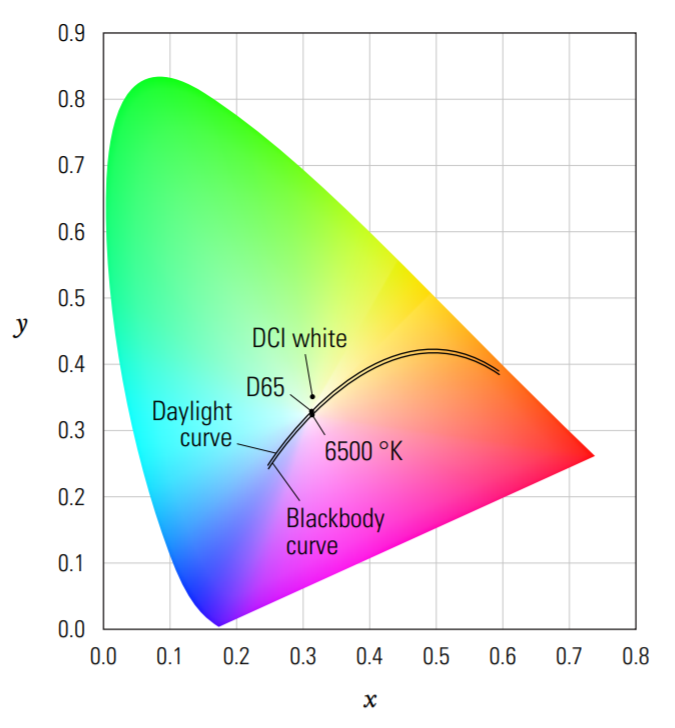
The daylight curve and the blackbody emission curve, while roughly parallel, are distinct.

Acknowledgements

Illustrations by Kazunori Tanaka. A very special thanks goes to:

Sony Pictures Imageworks
Rob Bredow, for this opportunity to contribute in a public forum.
Erik Strauss, Bob Peitzman, the Katana team, and Imageworks artists.
All contributors to OpenColorIO, including Malcolm Humphreys, Ben Dickson, Mark Fickett, Brian Hall, and Sean Looper.
The Foundry
The Academy s Scientific and Technical Council, including Ray Feeney, Alex Forsythe, and Andy Maltz.
Josh Pines, Stefan Luka, Alex, and Joseph Slomka
The Visual Effects Society

About the Author

Jeremy Selan is an Imaging Supervisor at Sony Pictures Imageworks specializing in color, lighting, and compositing. His work has been used on dozens of motion pictures including The Amazing Spider-Man, Alice in Wonderland, and The Smurfs. Jeremy is a co-founder of Katana, and also the founder of OpenColorIO. His work on color processing has been previously featured in GPU Gems 2, Siggraph 2005’s Electronic Theater, and the 2012 Siggraph Course, Cinematic Color.

References & Further Reading

Books

Ansel Adams — The Camera, Book 1. Little, Brown, and Company.
Ansel Adams — The Negative, Book 2. Little, Brown, and Company.
Ansel Adams — The Print, Book 3. Little, Brown, and Company.
Jim Blinn — Jim Blinn s Corner: Dirty Pixels. Morgan Kaufmann.
Mark Fairchild — Color Appearance Models. Addison-Wesley.
Ed Giorgianni — Digital Color Management: Encoding Solutions. Prentice Hall. Glenn Kennel — Color and Mastering for Digital Cinema. Focal Press.
R.W.G. Hunt — Measuring Colour. Fountain Press.
Charles Poynton — A Technical Introduction to Digital Video. Wiley. Erik Reinhard et al. — Color Imaging, Fundamentals and Applications. AK Peters, Ltd. Gunter Wyszecki & W.S. Stiles— Color Science: Concepts and Methods. Wiley & Sons, Inc.

Papers

Porter & Duff, Compositing Digital Images. Computer Graphics Volume 18. pp. 253-259. 1984.
Giorgianni, Ed. Color Management for Digital Cinema: A Proposed Architecture and Methodology for Creating, Encoding, Storing and Displaying Color Images in Digital Cinema Systems. Submitted to the Science and Technology Council, Academy of Motion Picture Arts and Sciences. 2005.

Online

Cinematic Color Download this document, and others, related to motion-picture color management
Bruce Lindbloom - Online resource for color conversion math
Charles Poynton Information for video standards and gamma, available for download.
DCI Specification Standards for theatrical digital distribution and colorimetry.
DCraw - Free, high quality, camera raw convertor
OpenColorIO Open-source color management framework for visual effects and animation
Visualizing the XYZ Color Space (YouTube) - Visual exploration of CIE XYZ
Reflecting Mapping HistoryA retrospective by Paul Debevec on reflection mapping

Published by The Visual Effects Society with the permission of Sony Pictures Imageworks and the author.