Fourier transform
Description
In physics and mathematics, the Fourier transform (FT) is a transform that converts a function into a form that describes the frequencies present in the original function. The output of the transform is a complex-valued function of frequency. The term Fourier transform refers to both this complex-valued function and the mathematical operation. When a distinction needs to be made the Fourier transform is sometimes called the frequency domain representation of the original function. The Fourier transform is analogous to decomposing the sound of a musical chord into terms of the intensity of its constituent pitches.
Fast Fourier transform
FFT
Theory
Fourier Transform is used to analyze the frequency characteristics of various filters. For images, 2D Discrete Fourier Transform (DFT) is used to find the frequency domain. A fast algorithm called Fast Fourier Transform (FFT) is used for calculation of DFT. Details about these can be found in any image processing or signal processing textbooks. Please see Additional Resources_ section.
For a sinusoidal signal, x(t)=Asin(2πft), we can say f is the frequency of signal, and if its frequency domain is taken, we can see a spike at f. If signal is sampled to form a discrete signal, we get the same frequency domain, but is periodic in the range [−π,π] or [0,2π] (or [0,N] for N-point DFT). You can consider an image as a signal which is sampled in two directions. So taking fourier transform in both X and Y directions gives you the frequency representation of image.
More intuitively, for the sinusoidal signal, if the amplitude varies so fast in short time, you can say it is a high frequency signal. If it varies slowly, it is a low frequency signal. You can extend the same idea to images. Where does the amplitude varies drastically in images ? At the edge points, or noises. So we can say, edges and noises are high frequency contents in an image. If there is no much changes in amplitude, it is a low frequency component. ( Some links are added to Additional Resources_ which explains frequency transform intuitively with examples).
Fourier Transform in Numpy
First we will see how to find Fourier Transform using Numpy. Numpy has an FFT package to do this. np.fft.fft2() provides us the frequency transform which will be a complex array. Its first argument is the input image, which is grayscale. Second argument is optional which decides the size of output array. If it is greater than size of input image, input image is padded with zeros before calculation of FFT. If it is less than input image, input image will be cropped. If no arguments passed, Output array size will be same as input.
Now once you got the result, zero frequency component (DC component) will be at top left corner. If you want to bring it to center, you need to shift the result by N2 in both the directions. This is simply done by the function, np.fft.fftshift(). (It is more easier to analyze). Once you found the frequency transform, you can find the magnitude spectrum.
import cv2 as cv
import numpy as np
from matplotlib import pyplot as plt
img = cv.imread('messi5.jpg',0)
f = np.fft.fft2(img)
fshift = np.fft.fftshift(f)
magnitude_spectrum = 20*np.log(np.abs(fshift))
plt.subplot(121),plt.imshow(img, cmap = 'gray')
plt.title('Input Image'), plt.xticks([]), plt.yticks([])
plt.subplot(122),plt.imshow(magnitude_spectrum, cmap = 'gray')
plt.title('Magnitude Spectrum'), plt.xticks([]), plt.yticks([])
plt.show()
Result look like below:
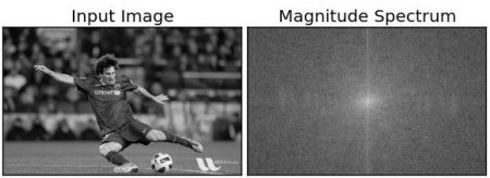
See, You can see more whiter region at the center showing low frequency content is more.
So you found the frequency transform Now you can do some operations in frequency domain, like high pass filtering and reconstruct the image, ie find inverse DFT. For that you simply remove the low frequencies by masking with a rectangular window of size 60x60. Then apply the inverse shift using np.fft.ifftshift() so that DC component again come at the top-left corner. Then find inverse FFT using np.ifft2() function. The result, again, will be a complex number. You can take its absolute value.
rows, cols = img.shape
crow,ccol = rows//2 , cols//2
fshift[crow-30:crow+31, ccol-30:ccol+31] = 0
f_ishift = np.fft.ifftshift(fshift)
img_back = np.fft.ifft2(f_ishift)
img_back = np.real(img_back)
plt.subplot(131),plt.imshow(img, cmap = 'gray')
plt.title('Input Image'), plt.xticks([]), plt.yticks([])
plt.subplot(132),plt.imshow(img_back, cmap = 'gray')
plt.title('Image after HPF'), plt.xticks([]), plt.yticks([])
plt.subplot(133),plt.imshow(img_back)
plt.title('Result in JET'), plt.xticks([]), plt.yticks([])
plt.show()
Result look like below: